Introduction to image-based profiling with Pycytominer
Welcome! This tutorial introduces Pycytominer, a Python library for processing image-based profiling data from high-content microscopy experiments.
What You Will Learn
By the end of this tutorial, you will know how to:
Aggregate thousands of single-cell measurements into one representative profile per experimental well
Annotate profiles with experimental metadata, such as which compound was applied to each well
Normalize feature values to remove plate-to-plate technical variation
Select features to remove uninformative or redundant measurements
Build consensus profiles that collapse replicate experiments into a single representative vector
Background: What Is High-Content Microscopy?
High-content microscopy measures hundreds to thousands of informative phenotypic features that represent the morphology state of cells under different biological conditions (e.g., healthy vs. disease). High-content microscopy is often paired with high-throughput screening experiments that perturb cells with small-molecule compounds or genetic perturbations.
In a typical experiment:
Cells are grown in multi-well plates and treated with a panel of perturbations.
Optionally apply fluorescence dyes to stain distinct cellular compartments.
Automated microscopes capture hundreds of images per plate.
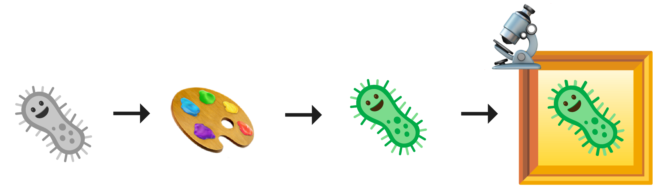
Image analysis software (such as CellProfiler) extracts several thousand numerical features per detected cell, describing each compartment’s and channel’s shape, texture, and fluorescence intensity.
A single experiment can generate measurements from millions of individual cells, spanning hundreds to thousands of features. The central challenge is transforming this raw, high-dimensional data into clean, interpretable image-based profiles — compact, comparable vectors that summarise how each condition changed the appearance of cells.
That is exactly what Pycytominer does (Serrano et al., 2025), which has been grounded in image-based profiling methods established over the past decade (Caicedo et al., 2017, Serrano et al. 2026).
Prerequisites
This tutorial assumes you have:
Familiarity with pandas DataFrames
(Optional) Completed the CytoTable tutorial, which shows how to convert raw CellProfiler output into the Parquet format that Pycytominer reads as input.
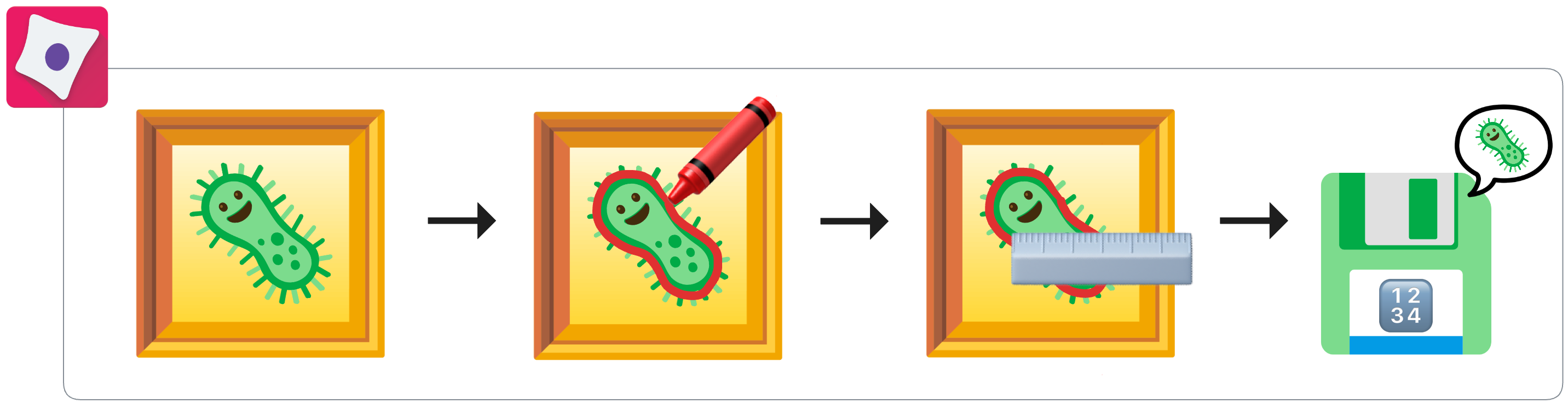
The Pycytominer Pipeline at a Glance
Raw single-cell data travels through five sequential steps:
Step |
Pycytominer function |
What changes |
|---|---|---|
|
|
One row per cell → one row per well |
|
|
Well positions → biological treatment labels |
|
|
Raw feature values → z-scores relative to controls |
|
|
Hundreds of features → only the informative ones |
|
|
One row per well → one row per treatment condition |
At the end, you have a compact, analysis-ready table where each row is a unique biological condition and each column is an informative morphological measurement.
[1]:
import numpy as np
import pandas as pd

from pycytominer import aggregate, annotate, consensus, feature_select, normalize

# Fix the random seed so this tutorial produces identical results every time it is run
np.random.seed(42)
Tutorial Data
In a real workflow, you would start from the Parquet file produced by CytoTable:
from pycytominer.cyto_utils import load_profiles

# Load single-cell measurements exported by CytoTable
single_cells = load_profiles("outputs/examplehuman.parquet")
For this tutorial we generate a small synthetic dataset that mirrors the exact structure of a real high-content microscopy experiment. The column names, data types, and naming conventions are identical to what CellProfiler and CytoTable produce — only the numerical values are simulated.
Experiment design:
Property |
Value |
|---|---|
Plates (biological replicates) |
2 |
Wells per plate |
6 (2 × DMSO vehicle control, 2 × Compound A, 2 × Compound B) |
Cells per well |
~100 |
Total single-cell measurements |
~1,200 |
Morphological features |
11 (across three compartments) |
Note on the features: Two of the eleven features are intentionally designed to be uninformative — one is constant across all cells, and one is nearly perfectly correlated with another. You will see these removed automatically in Step 4 (Feature Selection).
The simulation function is available in the expandable block below if you’d like to inspect it — you can skip it and go straight to Step 1.
def simulate_single_cells(plate_id, n_cells_per_well=100):
    """
    Generate synthetic single-cell morphology measurements for one plate.

    Column naming follows the CellProfiler convention:
      Metadata_*  — experimental context (plate, well, object identity)
      Cells_*     — measurements of the whole-cell boundary
      Cytoplasm_* — measurements of the cytoplasmic region
      Nuclei_*    — measurements of the nuclear region

    To keep this tutorial focused on the pipeline rather than biology,
    only the cell-area features respond to treatment. All other features
    are independent noise sampled from realistic distributions.
    In a real experiment every feature may carry some biological signal.
    """
    well_treatments = {
        'B02': 'DMSO',
        'C02': 'DMSO',
        'B03': 'Compound_A',
        'C03': 'Compound_A',
        'B04': 'Compound_B',
        'C04': 'Compound_B',
    }

    rows = []
    for image_number, (well, treatment) in enumerate(well_treatments.items(), start=1):
        is_a = float(treatment == 'Compound_A')
        is_b = float(treatment == 'Compound_B')

        # Only the Area family of features responds to treatment.
        # This ensures only the intentionally correlated pair is removed in Step 4.
        cell_area_base = np.random.normal(500 + 180 * is_a - 90 * is_b, 120, n_cells_per_well)

        for obj_num in range(1, n_cells_per_well + 1):
            cell_area = cell_area_base[obj_num - 1]
            rows.append({
                # ── Metadata columns ──────────────────────────────────────────
                'Metadata_Plate':        plate_id,
                'Metadata_Well':         well,
                'Metadata_ImageNumber':  image_number,
                'Metadata_ObjectNumber': obj_num,
                # ── Cell-level features ───────────────────────────────────────
                # Area and BoundingBoxArea are intentionally correlated (r ≈ 0.99);
                # one of the pair will be removed during feature selection.
                'Cells_AreaShape_Area':            cell_area,
                'Cells_AreaShape_BoundingBoxArea': cell_area * 1.3 + np.random.normal(0, 4),
                # EulerNumber = 1 for virtually all cells (topological invariant);
                # zero variance → removed during feature selection.
                'Cells_AreaShape_EulerNumber':     1,
                # All remaining features: independent noise with realistic distributions
                'Cells_AreaShape_Eccentricity':          float(np.clip(np.random.normal(0.55, 0.12), 0, 1)),
                'Cells_Intensity_MeanIntensity_Mito':    np.random.normal(0.30, 0.06),
                'Cells_Texture_Correlation_RNA_3_0_256': np.random.normal(0.22, 0.06),
                # ── Cytoplasm features ────────────────────────────────────────
                'Cytoplasm_AreaShape_Area':              np.random.normal(310, 80),
                'Cytoplasm_Intensity_MeanIntensity_AGP': np.random.normal(0.25, 0.07),
                # ── Nuclei features ───────────────────────────────────────────
                'Nuclei_AreaShape_Area':                 np.random.normal(195, 55),
                'Nuclei_AreaShape_Eccentricity':         float(np.clip(np.random.normal(0.40, 0.10), 0, 1)),
                'Nuclei_Intensity_MeanIntensity_DNA':    np.random.normal(0.50, 0.08),
            })
    return pd.DataFrame(rows)


# Generate data for two plates to simulate biological replicates
plate1 = simulate_single_cells('Plate_1')
plate2 = simulate_single_cells('Plate_2')
single_cells = pd.concat([plate1, plate2], ignore_index=True)

print(f'Single-cell dataset: {single_cells.shape[0]:,} rows (cells) x {single_cells.shape[1]} columns')
print(f'Plates:  {single_cells["Metadata_Plate"].unique().tolist()}')
print(f'Wells:   {sorted(single_cells["Metadata_Well"].unique().tolist())}')
print()
single_cells.head()
Step 1: Aggregate — From Cells to Wells
The single-cell table contains one row for every detected cell — in a real experiment this can easily reach hundreds of thousands of rows. However, biological interpretation happens at the level of the well (which treatment was applied), not the individual cell.
aggregate() summarises all cells within the same well into a single representative profile by computing the median of each feature across all cells in that well.
Parameter |
Description |
|---|---|
|
The single-cell DataFrame |
|
Columns that identify each well — cells sharing the same strata values are pooled together |
|
Automatically detect feature columns (any column whose name starts with a compartment prefix such as |
|
Summary statistic: |
[3]:
well_profiles = aggregate(
    population_df=single_cells,
    strata=["Metadata_Plate", "Metadata_Well"],
    features="infer",
    operation="median",
)

print(
    f"Single cells:  {single_cells.shape[0]:,} rows  →  Well profiles: {well_profiles.shape[0]} rows"
)
print(
    f"Columns:       {single_cells.shape[1]}          →               {well_profiles.shape[1]}"
)
print()
well_profiles
Single cells:  1,200 rows  →  Well profiles: 12 rows
Columns:       15          →               13
[3]:
| Metadata_Plate | Metadata_Well | Cells_AreaShape_Area | Cells_AreaShape_BoundingBoxArea | Cells_AreaShape_EulerNumber | Cells_AreaShape_Eccentricity | Cells_Intensity_MeanIntensity_Mito | Cells_Texture_Correlation_RNA_3_0_256 | Cytoplasm_AreaShape_Area | Cytoplasm_Intensity_MeanIntensity_AGP | Nuclei_AreaShape_Area | Nuclei_AreaShape_Eccentricity | Nuclei_Intensity_MeanIntensity_DNA | |
|---|---|---|---|---|---|---|---|---|---|---|---|---|---|
| 0 | Plate_1 | B02 | 484.765245 | 634.635906 | 1.0 | 0.532796 | 0.300860 | 0.216580 | 315.443258 | 0.263187 | 193.043658 | 0.418260 | 0.517625 |
| 1 | Plate_1 | B03 | 669.260838 | 870.994323 | 1.0 | 0.536427 | 0.304651 | 0.210215 | 314.055342 | 0.256479 | 190.671898 | 0.405648 | 0.498834 |
| 2 | Plate_1 | B04 | 399.970485 | 523.433308 | 1.0 | 0.533963 | 0.306359 | 0.222698 | 304.712780 | 0.252233 | 196.243981 | 0.394866 | 0.495179 |
| 3 | Plate_1 | C02 | 523.730623 | 685.309911 | 1.0 | 0.552298 | 0.307376 | 0.214065 | 328.921311 | 0.247123 | 197.812467 | 0.418402 | 0.489309 |
| 4 | Plate_1 | C03 | 671.001479 | 874.309123 | 1.0 | 0.557177 | 0.297985 | 0.212211 | 327.148733 | 0.235335 | 195.742017 | 0.406123 | 0.504755 |
| 5 | Plate_1 | C04 | 411.397559 | 535.575562 | 1.0 | 0.537410 | 0.296999 | 0.211021 | 307.751566 | 0.237890 | 187.333217 | 0.406370 | 0.501055 |
| 6 | Plate_2 | B02 | 510.859835 | 663.499468 | 1.0 | 0.560717 | 0.279879 | 0.210651 | 297.559100 | 0.245555 | 186.979153 | 0.395230 | 0.509640 |
| 7 | Plate_2 | B03 | 671.687004 | 869.272541 | 1.0 | 0.539517 | 0.310271 | 0.223312 | 323.749429 | 0.256434 | 193.420235 | 0.392844 | 0.503184 |
| 8 | Plate_2 | B04 | 420.512564 | 542.359150 | 1.0 | 0.556893 | 0.309685 | 0.215100 | 297.933806 | 0.239380 | 185.984035 | 0.389872 | 0.498350 |
| 9 | Plate_2 | C02 | 515.312157 | 667.242484 | 1.0 | 0.571428 | 0.292990 | 0.219456 | 304.836628 | 0.249090 | 195.434170 | 0.387314 | 0.501398 |
| 10 | Plate_2 | C03 | 677.517456 | 882.379424 | 1.0 | 0.548610 | 0.296525 | 0.225144 | 295.410839 | 0.250994 | 197.704177 | 0.397884 | 0.514447 |
| 11 | Plate_2 | C04 | 407.760144 | 528.536944 | 1.0 | 0.514893 | 0.294377 | 0.209433 | 333.205131 | 0.251384 | 201.713063 | 0.417950 | 0.493228 |
Step 2: Annotate — Adding Experimental Context
After aggregation, each row represents a well, but the DataFrame only records where the measurement came from (plate and well position) — not what biological condition was in that well.
The connection between well positions and experimental conditions is stored in a plate map — a lookup table prepared by the researcher that records which compound, genetic perturbation, concentration, or other variable was assigned to each well.
annotate() merges the plate map onto the well profiles, adding a Metadata_ column for each piece of experimental information.
In real experiments, plate maps are usually supplied as CSV files from a Laboratory Information Management System (LIMS) or prepared manually. Here we create one directly as a DataFrame to show its structure.
First, let us define the plate map:
[4]:
# The plate map records the biological condition in each well position.
# The same layout was used for both plates in this experiment.
platemap = pd.DataFrame({
    # 'well_position' is the standard column name expected by annotate()
    "well_position": ["B02", "C02", "B03", "C03", "B04", "C04"],
    "treatment": [
        "DMSO",
        "DMSO",
        "Compound_A",
        "Compound_A",
        "Compound_B",
        "Compound_B",
    ],
    "cell_line": ["HeLa"] * 6,
    "concentration_um": [0.0, 0.0, 10.0, 10.0, 10.0, 10.0],
})

print("Plate map:")
platemap
Plate map:
[4]:
| well_position | treatment | cell_line | concentration_um | |
|---|---|---|---|---|
| 0 | B02 | DMSO | HeLa | 0.0 |
| 1 | C02 | DMSO | HeLa | 0.0 |
| 2 | B03 | Compound_A | HeLa | 10.0 |
| 3 | C03 | Compound_A | HeLa | 10.0 |
| 4 | B04 | Compound_B | HeLa | 10.0 |
| 5 | C04 | Compound_B | HeLa | 10.0 |
[5]:
# annotate() joins the plate map onto the well profiles.
#
# join_on specifies [platemap_column, profiles_column] used for matching wells.
# add_metadata_id_to_platemap=True prepends 'Metadata_' to all plate map column names,
# following the pycytominer convention that all non-feature columns start with 'Metadata_'.
annotated_profiles = annotate(
    profiles=well_profiles,
    platemap=platemap,
    join_on=["Metadata_well_position", "Metadata_Well"],
    add_metadata_id_to_platemap=True,
)

print(
    f"Annotated profiles: {annotated_profiles.shape[0]} rows x {annotated_profiles.shape[1]} columns"
)
print()

# Show the metadata columns that were added
meta_cols = [
    "Metadata_Plate",
    "Metadata_Well",
    "Metadata_treatment",
    "Metadata_cell_line",
    "Metadata_concentration_um",
]
print("Well-to-treatment mapping after annotation:")
annotated_profiles[meta_cols].drop_duplicates().sort_values("Metadata_Well")
Annotated profiles: 12 rows x 16 columns

Well-to-treatment mapping after annotation:
[5]:
| Metadata_Plate | Metadata_Well | Metadata_treatment | Metadata_cell_line | Metadata_concentration_um | |
|---|---|---|---|---|---|
| 0 | Plate_1 | B02 | DMSO | HeLa | 0.0 |
| 1 | Plate_2 | B02 | DMSO | HeLa | 0.0 |
| 4 | Plate_1 | B03 | Compound_A | HeLa | 10.0 |
| 5 | Plate_2 | B03 | Compound_A | HeLa | 10.0 |
| 8 | Plate_1 | B04 | Compound_B | HeLa | 10.0 |
| 9 | Plate_2 | B04 | Compound_B | HeLa | 10.0 |
| 2 | Plate_1 | C02 | DMSO | HeLa | 0.0 |
| 3 | Plate_2 | C02 | DMSO | HeLa | 0.0 |
| 6 | Plate_1 | C03 | Compound_A | HeLa | 10.0 |
| 7 | Plate_2 | C03 | Compound_A | HeLa | 10.0 |
| 10 | Plate_1 | C04 | Compound_B | HeLa | 10.0 |
| 11 | Plate_2 | C04 | Compound_B | HeLa | 10.0 |
Step 3: Normalize — Removing Technical Variation
CellProfiler features differ widely in scale and units. For example:
Cells_AreaShape_Areamight range from 200 to 1,000 (pixels²)Nuclei_Intensity_MeanIntensity_DNAmight range from 0.1 to 0.9 (arbitrary fluorescence units)
Without normalization, features with large absolute values would dominate any downstream distance calculation or machine-learning model, regardless of whether they carry biological signal. Normalization also corrects for plate-to-plate technical variation caused by differences in staining efficiency, imaging conditions, or cell density between experimental batches.
normalize() rescales each feature using the distribution of control wells as a reference. The default method ('standardize') subtracts the control mean and divides by the control standard deviation — a standard z-score transformation. After normalization, control wells cluster around zero, and treated wells are expressed in units of standard deviations away from the control.
What is a vehicle control? DMSO (dimethyl sulfoxide) is the standard solvent used to dissolve most small-molecule compounds. Adding DMSO at the same concentration as the compound solvent, but without any active compound, defines the biological baseline — what cells look like when nothing meaningful has been done to them.
Parameter |
Description |
|---|---|
|
A pandas query string selecting the control wells used to compute normalization statistics |
|
|
[6]:
normalized_profiles = normalize(
    profiles=annotated_profiles,
    features="infer",
    meta_features="infer",
    samples="Metadata_treatment == 'DMSO'",  # use DMSO wells as the normalization reference
    method="standardize",
)

print(f"Normalized profiles: {normalized_profiles.shape}")

# Sanity check: DMSO wells should be centred near 0 after normalization
feature_cols = [c for c in normalized_profiles.columns if not c.startswith("Metadata_")]
dmso_rows = normalized_profiles["Metadata_treatment"] == "DMSO"

print()
print("Mean feature values in DMSO wells (should be ≈ 0.0 after normalization):")
print(normalized_profiles.loc[dmso_rows, feature_cols].mean().round(3).to_string())
Normalized profiles: (12, 16)

Mean feature values in DMSO wells (should be ≈ 0.0 after normalization):
Cells_AreaShape_Area                     0.0
Cells_AreaShape_BoundingBoxArea         -0.0
Cells_AreaShape_EulerNumber              0.0
Cells_AreaShape_Eccentricity             0.0
Cells_Intensity_MeanIntensity_Mito       0.0
Cells_Texture_Correlation_RNA_3_0_256    0.0
Cytoplasm_AreaShape_Area                -0.0
Cytoplasm_Intensity_MeanIntensity_AGP    0.0
Nuclei_AreaShape_Area                    0.0
Nuclei_AreaShape_Eccentricity           -0.0
Nuclei_Intensity_MeanIntensity_DNA      -0.0
Step 4: Feature Selection — Keeping Only Informative Features
A typical high-content microscopy dataset contains 500–1,500 features per well. Many of these features carry little or no biological information and can actively harm downstream analyses by adding noise:
Constant or near-constant features have the same value in every well and therefore cannot distinguish one treatment from another.
Highly correlated features (e.g.,
Cells_AreaShape_AreaandCells_AreaShape_BoundingBoxArea) measure essentially the same property through slightly different calculations. Retaining both adds redundancy without adding biological information.Blocklisted features are features empirically identified as technically unreliable across many published CellProfiler pipelines.
feature_select() applies these removal criteria in sequence:
Operation |
What it removes |
|---|---|
|
Features with variance below a minimum threshold (effectively constant) |
|
One feature from every highly correlated pair (Pearson r > 0.9) |
|
Features on the community-curated Pycytominer blocklist |
Recall from the data generation step that we deliberately included two uninformative features:
Cells_AreaShape_EulerNumber— constant (= 1) for all cells → removed byvariance_thresholdCells_AreaShape_Area/Cells_AreaShape_BoundingBoxArea— nearly perfectly correlated (r ≈ 0.99) → one of the pair is removed bycorrelation_threshold
Which of the correlated pair is kept? The algorithm retains the feature with the lower average correlation to all other features.
[7]:
selected_profiles = feature_select(
    profiles=normalized_profiles,
    features="infer",
    operation=["variance_threshold", "correlation_threshold", "blocklist"],
)

feature_cols_before = [
    c for c in normalized_profiles.columns if not c.startswith("Metadata_")
]
feature_cols_after = [
    c for c in selected_profiles.columns if not c.startswith("Metadata_")
]

print(f"Features before selection: {len(feature_cols_before)}")
print(f"Features after  selection: {len(feature_cols_after)}")
print(
    f"Features removed:          {len(feature_cols_before) - len(feature_cols_after)}"
)
print()
print("Retained features:")
for col in sorted(feature_cols_after):
    print(f"  {col}")
Features before selection: 11
Features after  selection: 9
Features removed:          2

Retained features:
  Cells_AreaShape_BoundingBoxArea
  Cells_AreaShape_Eccentricity
  Cells_Intensity_MeanIntensity_Mito
  Cells_Texture_Correlation_RNA_3_0_256
  Cytoplasm_AreaShape_Area
  Cytoplasm_Intensity_MeanIntensity_AGP
  Nuclei_AreaShape_Area
  Nuclei_AreaShape_Eccentricity
  Nuclei_Intensity_MeanIntensity_DNA
Step 5: Consensus — Collapsing Replicates
At this point we have one profile per well. Because our experiment was run across two plates (biological replicates), we have four profiles for each treatment condition — two wells per plate times two plates. Some downstream analyses expect a single, definitive profile per condition.
consensus() collapses replicate profiles into one consensus profile per treatment group by computing the median across all replicates.
Using the consensus profile instead of individual replicates:
Reduces the influence of plate-specific technical artefacts that survived normalization
Produces a lower-variance, higher-confidence representation of the treatment effect
Simplifies downstream analysis by reducing the number of rows to cluster or classify
The replicate_columns parameter specifies which metadata columns define a unique condition. Profiles that share the same values in these columns are treated as replicates and collapsed into a single consensus row.
[8]:
consensus_profiles = consensus(
    profiles=selected_profiles,
    replicate_columns=[
        "Metadata_treatment",
        "Metadata_cell_line",
        "Metadata_concentration_um",
    ],
    operation="median",
    features="infer",
)

print(f"Profiles before consensus: {selected_profiles.shape[0]} rows  (one per well)")
print(
    f"Profiles after  consensus: {consensus_profiles.shape[0]} rows  (one per treatment)"
)
print()
consensus_profiles
Profiles before consensus: 12 rows  (one per well)
Profiles after  consensus: 3 rows  (one per treatment)
[8]:
| Metadata_treatment | Metadata_cell_line | Metadata_concentration_um | Cells_AreaShape_BoundingBoxArea | Cells_AreaShape_Eccentricity | Cells_Intensity_MeanIntensity_Mito | Cells_Texture_Correlation_RNA_3_0_256 | Cytoplasm_AreaShape_Area | Cytoplasm_Intensity_MeanIntensity_AGP | Nuclei_AreaShape_Area | Nuclei_AreaShape_Eccentricity | Nuclei_Intensity_MeanIntensity_DNA | |
|---|---|---|---|---|---|---|---|---|---|---|---|---|
| 0 | Compound_A | HeLa | 10.0 | 11.558693 | -0.724044 | 0.589681 | 0.794162 | 0.610831 | 0.353012 | 0.313659 | -0.219728 | -0.049983 |
| 1 | Compound_B | HeLa | 10.0 | -7.189962 | -1.316052 | 0.624929 | -0.656629 | -0.462245 | -0.835377 | -0.379430 | -0.302806 | -0.737681 |
| 2 | DMSO | HeLa | 0.0 | 0.148573 | 0.155330 | 0.160923 | 0.041498 | -0.131285 | -0.446743 | 0.228724 | 0.140684 | 0.097928 |
Summary
You have now processed a Cell Painting dataset through the complete Pycytominer pipeline. Here is a recap of what each step accomplished:
Step |
Function |
Rows |
Features |
|---|---|---|---|
Raw single-cell data |
— |
1,200 cells |
11 |
After |
pool cells per well |
12 wells |
11 |
After |
add treatment labels |
12 wells |
11 |
After |
z-score vs DMSO |
12 wells |
11 |
After |
remove uninformative features |
12 wells |
9 |
After |
collapse replicates |
3 conditions |
9 |
The final consensus_profiles DataFrame contains one row per biological treatment condition and nine informative morphological features — a compact, analysis-ready representation of how each treatment changed the appearance of cells.
Saving Your Profiles
Pycytominer provides cyto_utils.output() as its canonical function for writing profiles to disk — the same function each pipeline step calls internally when you pass an output_file argument. It handles compression, format selection, and file naming in one call, and supports four output types:
|
Extension |
Best for |
|---|---|---|
|
|
Gzip-compressed, readable by any tool |
|
|
Faster reads and smaller files for large screens |
|
|
|
|
|
Cloud-native AnnData storage |
from pycytominer.cyto_utils import output

# Gzip-compressed CSV (default) — small footprint, readable by any tool
output(
    df=consensus_profiles,
    output_filename="consensus_profiles.csv.gz",
    output_type="csv",
)

# Parquet — fast reads and efficient storage for large screens
output(
    df=consensus_profiles,
    output_filename="consensus_profiles.parquet",
    output_type="parquet",
)

# AnnData HDF5 — ready for scanpy, scverse, and single-cell workflows
output(
    df=consensus_profiles,
    output_filename="consensus_profiles.h5ad",
    output_type="anndata_h5ad",
)
Pro tip: Every pipeline function accepts an
output_fileargument that writes directly to disk and returns the file path instead of a DataFrame. This avoids storing intermediate results in memory for large datasets:consensus_profiles = consensus( profiles=selected_profiles, replicate_columns=["Metadata_treatment", "Metadata_cell_line", "Metadata_concentration_um"], operation="median", features="infer", output_file="consensus_profiles.parquet", output_type="parquet", ) # consensus_profiles is now the file path string, not a DataFrame
What to Do Next
With morphology profiles in hand, common next steps include:
Phenotypic clustering — group treatments by morphological similarity using hierarchical clustering or UMAP
Similarity analysis — identify compounds that produce the same cellular phenotype using correlation or cosine similarity metrics
Classification — train machine-learning models to predict a compound’s mechanism of action from its morphological profile
Dimensionality reduction — visualise the morphological space of an entire compound library in two dimensions using PCA or UMAP
Hit calling — identify which compounds produce a statistically significant morphological change relative to controls. copairs computes mean Average Precision (mAP) to score phenotypic activity and consistency at the well/profile level; Buscar operates directly on single-cell distributions to capture cellular heterogeneity and flag off-target effects
Further Reading
Pycytominer API Reference — full documentation for every function used in this tutorial
CytoTable tutorial — how to convert raw CellProfiler output into the Parquet format that Pycytominer reads
Cell Painting Gallery — a public repository of Cell Painting datasets ready for analysis
Pycytominer in the Wild
Pycytominer is used across some of the largest and most impactful image-based profiling initiatives in the world. Here are a few to spark your curiosity:
🧬 JUMP-CP — Joint Undertaking for Morphological Profiling
The largest public Cell Painting dataset ever produced, generated by a consortium of 13 pharmaceutical companies and academic institutions (including AstraZeneca, Bayer, Pfizer, Merck KGaA, and the Broad Institute). JUMP-CP profiled over 116,000 compounds and ~15,000 genetic perturbations, with all profiles processed using Pycytominer. The resulting resource is used to predict compound activity, identify drug mechanisms, and match small molecules to disease phenotypes — at industrial scale.
🔬 LINCS Cell Painting — Library of Integrated Network-based Cellular Signatures
An NIH-funded initiative that profiled 1,571 bioactive compounds across six doses and five replicates in A549 lung cancer cells. Pycytominer was adopted as the primary profiling tool for this dataset, producing normalized and feature-selected profiles (Levels 3–5) that are publicly available for download. LINCS demonstrated that image-based profiles could serve as a systematic, reproducible reference map of cellular responses to chemical perturbation.
🌍 EU-OPENSCREEN — European Chemical Biology Research Infrastructure
A distributed pan-European research infrastructure spanning 30 partner sites across eight countries. EU-OPENSCREEN has integrated Cell Painting into its screening platform, enabling European academic and industry researchers to access high-content imaging and morphological profiling as a service. Their contributions to the JUMP-CP consortium extended the reach of image-based profiling into the broader European drug discovery community.
🖼️ Cell Painting Gallery — Broad Institute Open Dataset Collection
A growing public repository of Cell Painting datasets, hosted on AWS as open data and maintained by the Carpenter–Singh and Cimini labs at the Broad Institute. The gallery spans tens of thousands of small-molecule treatments across diverse cell lines and experimental designs — all freely accessible and ready for analysis. It is the canonical reference point for new Cell Painting datasets produced by the community.
These resources process their raw CellProfiler outputs through the same Pycytominer pipeline you just ran — the only difference is scale.